Getting Started
API
SIMPL follows sklearn conventions: configure hyperparameters at init, pass data to fit().
from simpl import SIMPL

# 1. Configure the model (no data, no computation)
model = SIMPL(
    speed_prior=0.4,        # prior on agent speed (m/s) — controls Kalman smoothing
    kernel_bandwidth=0.02,  # KDE bandwidth for fitting receptive fields
    bin_size=0.02,          # spatial bin size for environment discretisation
    env_pad=0.0,            # padding around data bounds
)

# 2. Fit
model.fit(
    Y,                      # spike counts (T, N_neurons)
    Xb,                     # behavioural initialisation positions (T, D)
    time,                   # timestamps (T,)
    n_iterations=5,
    )

# 3. Access results
model.X_           # final decoded latent positions, shape (T, D)
model.F_           # final receptive fields, shape (N_neurons, *env_dims)
model.results_     # full xarray.Dataset with metrics, likelihoods, and baselines, across iterations.

# 4. Plot results
model.plot_fitting_summary()  # Shows bits-per-spike metric and spike-latent mutual information.

# (optional) Resume training if not yet converged
model.fit(Y, Xb, time, n_iterations=5, resume=True)
Prediction
Decode new spikes using the fitted receptive fields (no behavioural input needed). The new data must be binned at the same dt as the training data.
X_decoded = model.predict(Y_new)
model.prediction_results_  # xr.Dataset with rich results (mu_s, sigma_s, log-likelihoods, etc.)
Plotting
Built-in plotting methods provide quick diagnostics. All methods return matplotlib Axes for further customisation — for publication-quality figures, use model.results_ (an xarray.Dataset) to access the data directly.
# Log-likelihood and spatial information across iterations
model.plot_fitting_summary()

# Decoded trajectory (all iterations by default)
model.plot_latent_trajectory()
model.plot_latent_trajectory(time_range=(0, 60))  # zoom in, specific iterations

# Receptive fields (iteration 0 + last by default)
model.plot_receptive_fields(neurons=[0, 5, 10])

# Spike raster heatmap (time × neurons)
model.plot_spikes()
model.plot_spikes(time_range=(0, 60))

# Auto-discover and plot all per-iteration metrics
model.plot_all_metrics(show_neurons=False)

# Prediction on held-out data
model.predict(Y_test)
model.plot_prediction(Xb=Xb_test, Xt=Xt_test)
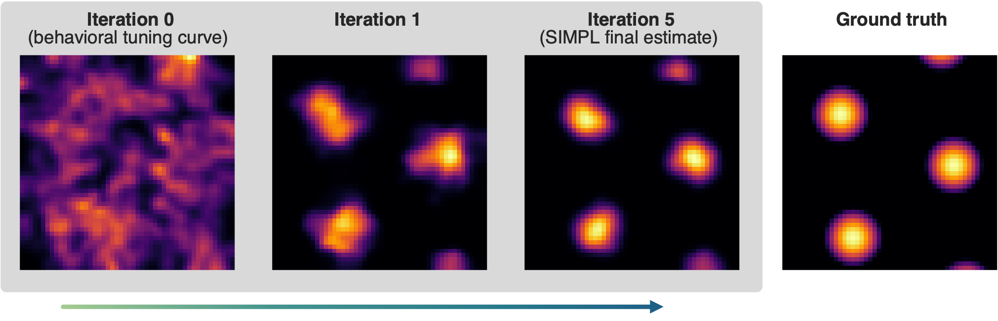
Synthetic grid cell tuning curves optimised from a noisy behavioural initialisation
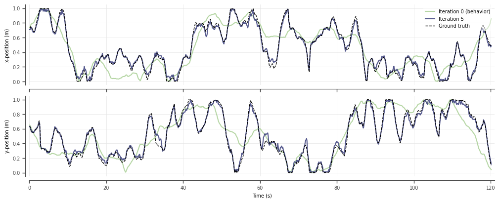
True latent trajectory recovered by SIMPL

Bits-per-spike and mutual-information metrics improve across epochs and exceed naive ML
Saving and loading
model.save_results("results.nc")

# Load results as an xr.Dataset for custom analysis
from simpl import load_results
results = load_results("results.nc")

# Or rehydrate a full model for plotting, prediction, or resumed training
# (constructor arguments must exactly match the original training run)
model = SIMPL(speed_prior=0.4, kernel_bandwidth=0.025, bin_size=0.02)
model.load("results.nc")
model.fit(Y, Xb, time, n_iterations=5, resume=True)  # pick up where you left off
Ground truth baselines
If you have ground truth positions (and optionally ground truth receptive fields), register them before fitting so that baseline metrics (latent R2, field error, etc.) are computed at each iteration:
model.add_baselines(Xt=Xt, Ft=Ft, Ft_coords_dict={"y": ybins, "x": xbins})
model.fit(Y, Xb, time, n_iterations=5)  # baselines computed automatically
1D angular / circular data
SIMPL supports 1D circular latent variables (e.g. head direction) via the is_1D_angular flag. When enabled, the environment is fixed to [-π, π), angular KDE is used for receptive fields, and the Kalman filter wraps its state to [-π, π) after every predict, update, and smooth step.
model = SIMPL(
    is_1D_angular=True,
    bin_size=np.pi / 32,
    env_pad=0.0,
    speed_prior=0.1,
    kernel_bandwidth=0.3,
)
model.fit(Y, Xb, time, n_iterations=5)  # Xb should be in radians, [-pi, pi)
Note: The wrapped Kalman filter assumes a tight posterior (σ ≪ 2π). If posterior uncertainty is large relative to the circular domain, decoding accuracy may degrade.
Trial boundaries
When data comes from multiple recording sessions or trials, you don't want the Kalman smoother blending across discontinuities. Pass trial_boundaries — an array of time-bin indices where each new trial starts — and SIMPL will run the filter/smoother independently within each segment. The initial state for each trial is estimated from the likelihood modes within that trial.
# Three trials starting at time-bins 0, 5000, and 12000
model.fit(Y, Xb, time, n_iterations=5, trial_boundaries=[0, 5000, 12000])
If your timestamps have gaps (e.g. concatenated sessions), SIMPL will warn you and suggest using trial_boundaries to avoid smoothing across the jumps.
GPU acceleration
SIMPL auto-detects and offloads compute-heavy steps to GPU when available. Typical neural recordings (< 2 hrs) fit in under 60 s on CPU alone, so a GPU is rarely needed.
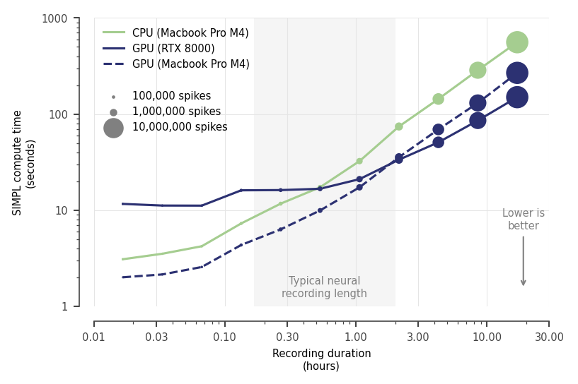
200 neurons, dt=0.02s (50Hz), dx=2cm (2,500 bins), 5 iterations, includes JIT overheads
pip install -U "jax[cuda12]"   # NVIDIA GPU (CUDA)
pip install ".[metal]"           # Apple Silicon GPU (experimental and not recommended, pins JAX to 0.4.35)
model = SIMPL(use_gpu=False) # force CPU
Data preprocessing utilities
from simpl import accumulate_spikes, coarsen_dt

# Roll up spikes into wider time bins (e.g. sum every 2 bins)
Y_coarse, Xb_coarse, time_coarse = coarsen_dt(Y, Xb, time, dt_multiplier=2)

# Accumulate spikes with a causal sliding window
Y_accum = accumulate_spikes(Y, window=3)
Examples
The examples/simpl_demo.ipynb notebook walks through the full SIMPL workflow across four datasets:
- Synthetic grid cells — fits SIMPL on artificial grid cell data with known ground truth, demonstrating decoded trajectories, receptive field recovery, log-likelihood improvements, and prediction on held-out data.
- Real place cells — fits SIMPL on real hippocampal place cell recordings from Tanni et al. (2022), where no ground truth is available.
- Real head direction cells — fits SIMPL in 1D angular mode on head direction cell recordings from Vollan et al. (2025), demonstrating circular latent variable decoding and polar receptive field plots.
- Motor cortex hand reaching — fits SIMPL on somatosensory cortex recordings from Chowdhury et al. (2020), demonstrating higher-dimensional latent variables (2D and 4D) and model comparison across different behavioural initialisations (position vs velocity vs combined).
![]()