Advanced Usage
Saving and loading
model.save_results("results.nc")

# Load results as an xr.Dataset for custom analysis
from simpl import load_results

results = load_results("results.nc")

# Or rehydrate a full model for plotting, prediction, or resumed training
# (constructor arguments must exactly match the original training run)
model = SIMPL(speed_prior=0.4, kernel_bandwidth=0.025, bin_size=0.02)
model.load("results.nc")
model.fit(Y, Xb, time, n_iterations=5, resume=True)  # pick up where you left off
Ground truth baselines
If you have ground truth positions (and optionally ground truth receptive fields), register them before fitting so that baseline metrics (latent R2, field error, etc.) are computed at each iteration:
model.add_baselines(Xt=Xt, Ft=Ft, Ft_coords_dict={"y": ybins, "x": xbins})
model.fit(Y, Xb, time, n_iterations=5)  # baselines computed automatically
Temporal vs. non-temporal datasets
Temporal structure enters SIMPL only through the Kalman smoothing prior. A temporal dataset might be hippocampal navigation, where neighboring samples are adjacent moments in an animal's trajectory and smoothness over time is meaningful. A non-temporal dataset might be neural responses to visual stimuli, where each point is a separate trial and neighboring rows do not imply temporal continuity.
Once Kalman smoothing is disabled, SIMPL is, in effect, iterative maximum likelihood: each observation is decoded independently from the current receptive fields, then the receptive fields are refit from those decoded positions.
If your samples do not have meaningful time stamps or temporal ordering, pass time=None when calling fit():
model = SIMPL(speed_prior=None)
model.fit(Y, Xb, time=None)
When time=None, SIMPL treats the data as non-temporal, replaces the missing time coordinate with np.arange(T), and forcefully disables Kalman smoothing. In this setting, the saved time coordinate is better interpreted as trial/sample index rather than physical time.
1D angular / circular data
SIMPL supports 1D circular latent variables (e.g. head direction) via the is_1D_angular flag. When enabled, the environment is fixed to [-π, π), angular KDE is used for receptive fields, and the Kalman filter wraps its state to [-π, π) after every predict, update, and smooth step. Do not set env_lims or a nonzero env_pad in angular mode.
model = SIMPL(
    is_1D_angular=True,
    bin_size=np.pi / 32,
    speed_prior=0.1,
    kernel_bandwidth=0.3,
)
model.fit(Y, Xb, time, n_iterations=5)  # Xb should be in radians, [-pi, pi)
Note: The wrapped Kalman filter assumes a tight posterior (σ ≪ 2π). If posterior uncertainty is large relative to the circular domain, decoding accuracy may degrade.
Trial boundaries
When data comes from multiple recording sessions or trials, you don't want the Kalman smoother blending across discontinuities. Pass trial_boundaries — an array of time-bin indices marking where each new trial starts — and SIMPL will run the filter/smoother independently within each segment. The initial state for each trial is estimated from the likelihood modes within that trial.
# Three trials starting at time-bins 0, 5000, and 12000
model.fit(Y, Xb, time, n_iterations=5, trial_boundaries=[0, 5000, 12000])
If your timestamps have gaps (e.g. concatenated sessions), SIMPL will warn you and suggest using trial_boundaries to avoid smoothing across the jumps.
GPU Acceleration
SIMPL auto-detects and offloads compute-heavy steps to GPU when available. Most typical neural recordings fit in under 60 s on CPU alone, so a GPU is rarely needed.
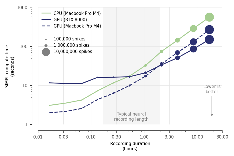
200 neurons, dt=0.02s (50Hz), dx=2cm (2,500 bins), 5 iterations, includes JIT overheads
Choose exactly one installation path:
# CPU (recommended; macOS, Linux, or Windows)
pip install simpl-neuro

# NVIDIA CUDA 12 (Linux/Windows only)
pip install -U "jax[cuda12]"
pip install simpl-neuro

# Apple Silicon Metal (experimental)
pip install "simpl-neuro[metal]"
Do not install the CUDA extra on macOS.
pip install --force-reinstall "simpl-neuro[metal]"
# Local editable checkout:
pip install --force-reinstall -e ".[metal]"
model = SIMPL()  # use a GPU when available (default)
model = SIMPL(use_gpu=False)  # force CPU
model = SIMPL(use_gpu=True)  # require a GPU
With use_gpu=False, SIMPL selects CPU directly without initialising installed
GPU or Metal backends.
Data preprocessing utilities
from simpl import accumulate_spikes, coarsen_dt

# Roll up spikes into wider time bins (e.g. sum every 2 bins)
Y_coarse, Xb_coarse, time_coarse = coarsen_dt(Y, Xb, time, dt_multiplier=2)

# Accumulate spikes with a causal sliding window
Y_accum = accumulate_spikes(Y, window=3)