Plotting and Metrics
Metrics
The four headline fitting metrics are:
- Spike log-likelihood (
logPYXF,logPYXF_val) — the mean Poisson log-likelihood of the observed spike counts under the fitted receptive fields evaluated along the decoded trajectory.We strongly suggest using
bits_per_spikeoverlogPYXFfor comparisons. Its zero point is interpretable, and the normalisation makes it easier to compare datasets with different neuron counts or recording lengths.
- Bits per spike (
bits_per_spike,bits_per_spike_val) — how much better the fitted tuning curves explain spikes than a mean-rate baseline, in bits per observed spike. This is useful for comparing fits across datasets with different spike counts or bin sizes:
- Skaggs spatial information (
spatial_information) — the standard spatial-information rate for each neuron, in bits/sec. It measures how informative the receptive field is about latent position in the small-time-bin limit:
Other metrics available in model.results_ include:
mutual_information— the exact finite-time-bin analog of spatial information, \(I(X;Y)\), in bits/s. It is the same idea as Skaggs spatial information, but computed from the full spike-count distribution rather than the small-bin approximation.X_R2,X_err— latent-position agreement with ground truth, whenXtis registered withadd_baselines.F_err— receptive-field error against ground-truth fields, whenFtis registered.field_change,trajectory_change— per-iteration changes in tuning curves and decoded trajectory.negative_entropy,sparsity— compactness/sparsity summaries of the fitted tuning curves.
For 2D environments, model.analyse_place_fields() adds morphology metrics to model.results_, including place-field count, size, position, roundness, and peak firing rate. This uses connected-component analysis on receptive fields and is not run automatically during fit().
Plotting
Built-in plotting methods provide quick diagnostics. All methods return matplotlib Axes for further customisation — to create figures from scratch, use model.results_ (an xarray.Dataset) to access the data directly.
# Log-likelihood and spatial information across iterations
model.plot_fitting_summary()

# Decoded trajectory (all iterations by default)
model.plot_latent_trajectory()
model.plot_latent_trajectory(time_range=60)  # first 60 seconds
model.plot_latent_trajectory(time_range=(0, 60), iterations=(0, 3, 5))  # zoom in, specific iterations

# Receptive fields (iteration 0 + last by default)
model.plot_receptive_fields(neurons=[0, 5, 10])

# Spike raster heatmap (time × neurons)
model.plot_spikes()
model.plot_spikes(time_range=(0, 60))

# Auto-discover and plot all per-iteration metrics
model.plot_all_metrics(show_neurons=False)

# 2D place-field morphology metrics
model.analyse_place_fields()

# Prediction on held-out data
model.predict(Y_test)
model.plot_prediction(
    Xb=Xb_test,
    Xt=Xt_test,  # Xt_test is optional ground truth for the prediction data
)
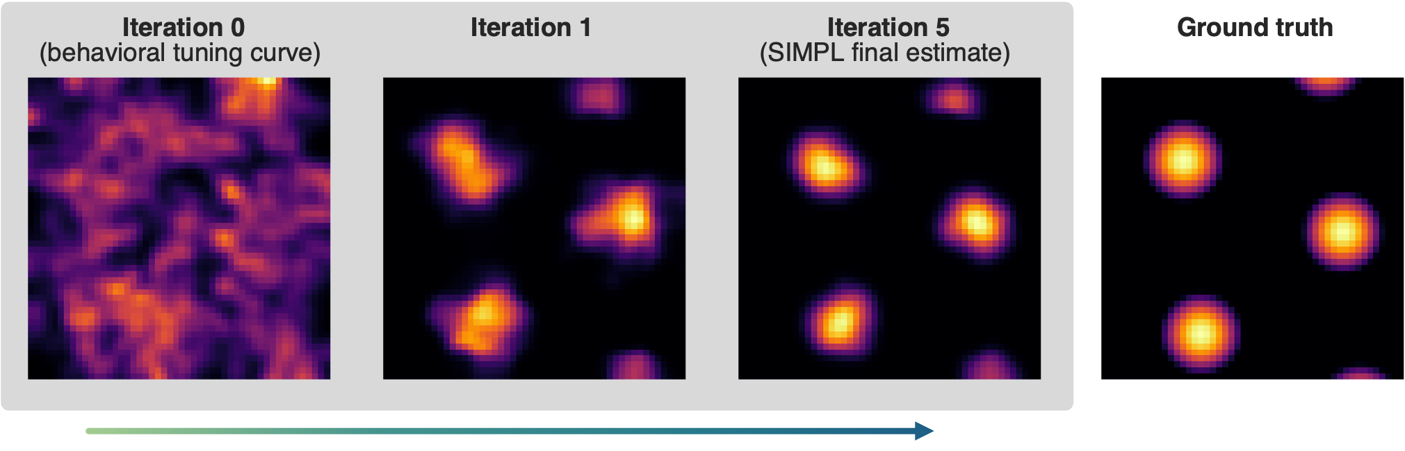
Synthetic grid cell tuning curves optimised from a noisy behavioural initialisation
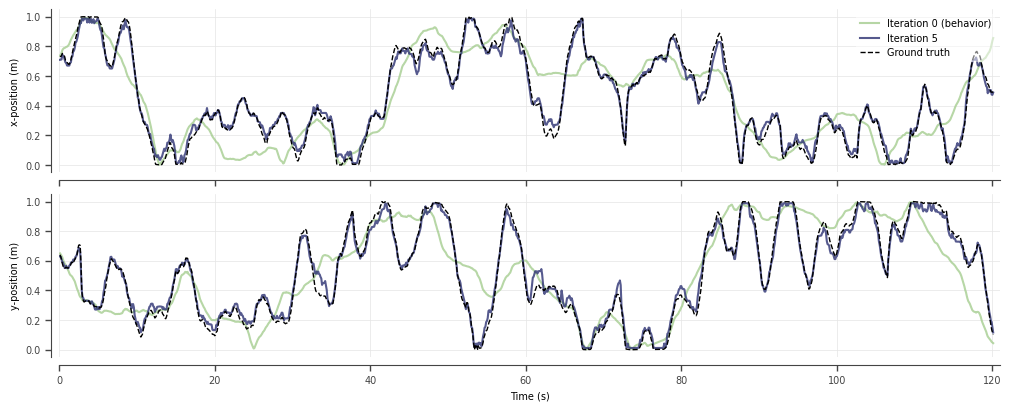
True latent trajectory recovered by SIMPL

Bits-per-spike and mutual-information metrics improve across epochs and exceed naive ML